Causal Machine Learning in Healthcare
Introduction
Causal inference is core to medicine. In this setting, we generally have
some covariates (e.g., age, gender, images) about a patient and want to
answer the counterfactual (Pearl and Mackenzie 2018) question: Which
treatment would lead to the best outcome? The state of the art approach
to answer this question are randomised controlled trials (RCTs) (Hariton
and Locascio 2018) in which patients are assigned to the intervention or
the comparator group at random. If the sample size is large enough, the
act of randomization ensures that potential confounders (measured and
unmeasured) are balanced between the groups which allows the attribution
of differences in the outcome to the intervention. However, researchers
face several challenges when conducting these trials:
-
Representativeness/Generalisation: The study is only applicable to large groups in the real world if the original population of the trial is representative. There may be biases in the population (e.g., because of the recruitment process) that decrease generalization.
-
Costs/Resources: RCTs are very expensive and require experts and manual labor. In 2013, the average per-patient costs were estimated at $36,500 per trial phase and developing a new medicine required an investment of around $2.6 billion (“Biopharmaceutical Industry-Sponsored Clinical Trials: Impact on State Economies” 2015).
-
Multiple Treatments: We often want to compare more than one treatment.
-
Measuring Outcomes: For some diseases, measuring the outcome can be hard, for instance because the effects are only observed after some years.
-
Ethical Issues: Not treating a patient can be unethical in some settings.
A second central application of causal inference in healthcare is the
discovery of interventions that could be used as new treatment options.
Currently, this is mainly done with experiments that are analyzed and
visualized, leading to new insights and experiments to further refine a
hypothesis. The problem with this approach is that it is manual and
largely driven by domain experts: Someone needs to come up with good
hypotheses, prioritise them, design the experiments, potentially merge
the evidence with other experiments, and decide if the results are
representative.
A key challenge when applying causal inference techniques to healthcare
is dealing with complexity. The causal generative process of the human
body is very sophisticated and the causal relations span multiple scales
of resolution, from reactions at the molecular level to symptoms of the
body as a whole. Furthermore, because of the previously mentioned
challenges with RCTs, addressing these problems by collecting more data
is often not feasible.
Estimating Causal Treatment Effects from Observations
Framework
We are in the Rubin-Neyman Potential Outcomes Framework (Rubin 2005)
in which there are
The population consists of
-
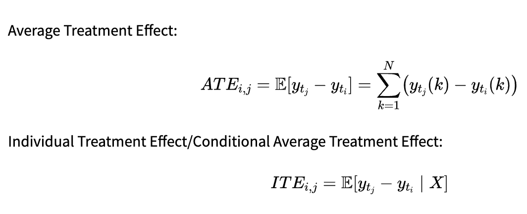
Average Treatment Effect:
-
Individual Treatment Effect/Conditional Average Treatment Effect:
The metric to use depends on our research question. ATE allows us to draw conclusions about the whole population: In our previous example, we could infer the average effect of smoking on the lung volume. On the other hand, ITE is useful for personalized recommendations. If we are able to infer it properly, we can decide which treatment is best for a patient based on the values.
For other research questions (e.g., estimating the difference between two groups of treatments and not the individual treatments), different metrics can be constructed based on the counterfactual outcomes, but ATE and ITE are most common in the literature.
Quasi-Experimental Studies
In quasi-experimental studies, we try to infer causal effects from
non-randomised experiments. While we can control for observed
confounding, we cannot do so for hidden (unmeasured) confounders. For
that reason, the degree of evidence for causal effects is generally
lower than in RCTs.
One type of quasi-experimental studies are case-control studies. The
outcomes across two groups are compared based on a potential causal
factor and we control for observed confounding by matching cases with
similar controls. Matching by comparing the covariates can be infeasible
because
-
Conditional Independence Assumption:
(with the special case ), meaning that the assignment of the treatment is independent of the outcome, given the balancing score. -
Common Support Assumption:
, i.e. every unit has a chance of receiving each treatment. -
Stable Unit Treatment Value Assumption (SUTVA): The values of all outcomes
are not affected by any (note that which value we observe in the study is obviously affected by , but the statement is about the whole vector which is partially unobserved), which implies that there is no interference between units.
These assumptions are generally untestable (Stone 1993), but Pearl
introduced a simple graphical test that can be applied to the causal
graph (which we need to construct with domain knowledge) for testing if
a set of variables is sufficient for identification (Pearl 1993).
Counterfactual Regression
Given the observational data, we want to train a counterfactual
estimator that allows us to predict (in Pearl’s
One approach is to learn individual models for the different treatments
(which can result in asymptotically consistent/unbiased estimates, e.g.
using the Double/Debiased Machine Learning approach introduced by
Chernozukov et al. (Chernozhukov et al. 2018), but this introduces
additional variance because the control and treated distributions (i.e.
Schwab et al. (Schwab, Linhardt, and Karlen 2019) extend TARNet to the
multiple treatment setting with
Dose-Response Networks (Schwab et al. 2020) are a further extension of
the described model architecture where the range of dosages is
discretized into buckets and a separate head layer is used for every
bucket. The number of buckets allows to tradeoff predictive performance
and computational requirements.
For the evaluation of counterfactual regression models that estimate the
ITE, the precision in estimating heterogenous effects (PEHE) is often
used, defined as (for binary treatments) (Hill 2011):
Where
Causal Explanation Models
We are often not only interested in the prediction of a model, but we
also want to know which inputs caused this prediction (i.e., calculate
feature importance scores for the different inputs). This is especially
important in healthcare because the interpretation of the output and the
further steps that are taken can depend a lot on the contributing
factors (in settings where humans and machine learning algorithms
cooperate). Furthermore, it can generally be beneficial for model
debugging as it allows to reason about the discovered patterns and judge
their reasonableness.
Attentive Mixture of Experts Model
One approach is to train machine-learning models that learn to jointly
produce accurate predictions and estimations of the feature importance,
for instance attentive mixture of experts (AME) models (Schwab,
Miladinovic, and Karlen 2018). The basic idea is to distribute the
features among experts (neural networks with their own
parameters/architectures, outputting their topmost feature
representation
Schwab et al. address this problem by introducing an objective function
that measures the mean Granger-causal error (MGE). In the
Granger-causality framework,
Comparison
An alternative approach for feature importance estimation is to model
the impact of local pertubations on the prediction (Adler et al. 2018).
The LIME (Local Interpretable Model-agnostic Explanations) algorithm
does this by sampling in a local region and fitting an interpretable
model (e.g., a sparse linear model) to these samples, which can help
understanding and validating the corresponding prediction (Ribeiro,
Singh, and Guestrin 2016). With multiple LIME explanations, the model as
a whole can be examined. SHAP (SHapley Additive exPlanations) calculates
the local feature importance using Shapley values (Shapley 1953), the
marginal contribution towards the reduction in prediction error
(Lundberg and Lee 2017). While both of these approaches are
model-agnostic, their sampling-based nature is computationally
demanding. AME shows similar estimation accuracy for the feature
importances with significantly lower computational requirements.
Furthermore, the associations identified by the AME model with a
properly tuned MGE/MSE tradeoff were consistent with those reported by
domain experts, which was not the case for the other evaluated models.
However, there are some limitations to AME models. The model structure
is fixed, which can result in worse predictive performance for certain
tasks. Moreover, as the MSE/MGE is jointly optimized, the MSE generally
increases when more importance is given to the MGE, meaning there is a
tradeoff between predictive performance and accurate importance
estimation. Furthermore, the direction of the influence (positive or
negative) is not inferred and with many features (and therefore experts,
if a one-to-one mapping is used), the optimization can become
intractable.
CXPlain Model
CXPlain addresses the issue of the fixed model structure and increasing
MSE that arises when using AME by training a separate explanation model
and allowing arbitrary predictive models (Schwab and Karlen 2019). The
explanation model treats the predictive models as blackboxes and
calculates its outputs with and without each input feature. Note that a
different strategy for obtaining the predictions without a feature is
needed than in AME models as the predictive model now is arbitrary and
cannot be modified. This can be accomplished by masking the feature with
zeroes, replacing it with the mean value, or using more sophisticated
masking schemes. Given these outputs, the (normalized) decrease in error
is calculated for every input feature and the Kullback-Leibler
divergence between this decrease and the models importance scores
Because some feature importance estimates may themselves be very
unreliable (Zhang et al. 2019), CXPlain additionally provides
uncertainty estimates for each feature importance estimate. It uses
bootstrap resampling for that, i.e. training the explanation model on
different subsets of the data (possibly containing duplicates) and using
the importance scores of the runs to construct confidence intervals.
As AME, CXPlain provided more accurate feature importance estimates than
LIME and SHAP, while being model-agnostic and still computationally
efficient. Even though the approach works with arbitrary models, the
accuracy of the estimates does depend on the predictive model and some
model architectures seem to be better suited for explanation models.
Conclusion
Although the problem statement of causal machine learning in healthcare is conceptually similar to other applications of causality in machine learning, the complexity is much higher. Much research is currently done on datasets with a few factors of variation and a relatively simple causal graph, such as robotics (Gondal 2019) or abstract reasoning on non-convoluted images (Locatello 2019). Because of the high complexity in the healthcare domain with very complicated relations and many causal factors, the current approaches often follow the pragmatic, task-solving based approach to causality: Instead of trying to infer all of the causal relationships (which may be very hard or even impossible to do for humans in healthcare), the goal is often to find useful, potentially causal relations that are helpful for solving tasks (that often involve humans).
It will be very interesting to see if we ever achieve a point where we are able to autonomously infer the causal graph in domains with such a high complexity and have enough confidence in the estimate to act upon it without human involvement. This would open up completely new possibilities such as cheap, personalized medicine and treatment procedures.
[1] Note that the term causality may be misleading in this context.
Because of that, some researchers use the term "predictive causality",
meaning a variable contains useful information for predicting another
(Diebold 2007). Granger himself later used the word "temporal relation"
instead of causality (C. Granger and Newbold 1986).
References
Adler, Philip, Casey Falk, Sorelle A. Friedler, Tionney Nix, Gabriel
Rybeck, Carlos Scheidegger, Brandon Smith, and Suresh
Venkatasubramanian. 2018. “Auditing Black-Box Models for Indirect
Influence.” Knowledge and Information Systems 54 (1): 95–122.
https://doi.org/10.1007/s10115-017-1116-3.
Bahdanau, Dzmitry, Kyunghyun Cho, and Yoshua Bengio. 2015. “Neural
Machine Translation by Jointly Learning to Align and Translate.” ICLR.
“Biopharmaceutical Industry-Sponsored Clinical Trials: Impact on State
Economies.” 2015. Pharmaceutical Research and Manufacturers of
America, March.
Chernozhukov, Victor, Denis Chetverikov, Mert Demirer, Esther Duflo,
Christian Hansen, Whitney Newey, and James Robins. 2018.
“Double/Debiased Machine Learning for Treatment and Structural
Parameters.” The Econometrics Journal 21 (1): C1–68.
https://doi.org/10.1111/ectj.12097.
Diebold, Francis X. 2007. Elements of Forecasting.
Thomson/South-Western.
Gondal, Muhammad Waleed, Manuel Wüthrich, ore Miladinović, Francesco
Locatello, Martin Breidt, Valentin Volchkov, Joel Akpo, Olivier Bachem,
Bernhard Schölkopf, and Stefan Bauer. 2019. “On the Transfer of
Inductive Bias from Simulation to the Real World: A New Disentanglement
Dataset.” arXiv:1906.03292 [Cs, Stat], November.
http://arxiv.org/abs/1906.03292.
Granger, C. W. J. 1969. “Investigating Causal Relations by Econometric
Models and Cross-Spectral Methods.” Econometrica 37 (3): 424–38.
https://doi.org/10.2307/1912791.
Granger, Clive, and Paul Newbold. 1986. “Forecasting Economic Time
Series.” Elsevier {{Monographs}}. Elsevier.
Hariton, Eduardo, and Joseph J. Locascio. 2018. “Randomised Controlled
Trialsthe Gold Standard for Effectiveness Research.” BJOG : An
International Journal of Obstetrics and Gynaecology 125 (13): 1716.
https://doi.org/10.1111/1471-0528.15199.
Hill, Jennifer L. 2011. “Bayesian Nonparametric Modeling for Causal
Inference.” Journal of Computational and Graphical Statistics 20 (1):
217–40. https://doi.org/10.1198/jcgs.2010.08162.
Lechner, Michael. 2001. “Identification and Estimation of Causal Effects
of Multiple Treatments Under the Conditional Independence Assumption.”
In Econometric Evaluation of Labour Market Policies, edited by Michael
Lechner and Friedhelm Pfeiffer, 43–58. ZEW Economic Studies. Heidelberg:
Physica-Verlag HD. https://doi.org/10.1007/978-3-642-57615-7_3.
Locatello, Francesco, Stefan Bauer, Mario Lucic, Gunnar Raetsch, Sylvain
Gelly, Bernhard Schölkopf, and Olivier Bachem. 2019. “Challenging Common
Assumptions in the Unsupervised Learning of Disentangled
Representations.” In International Conference on Machine Learning,
4114–24.
Lundberg, Scott M., and Su-In Lee. 2017. “A Unified Approach to
Interpreting Model Predictions.” Advances in Neural Information
Processing Systems 30: 4765–74.
Pearl, Judea. 1993. “Bayesian Analysis in Expert Systems: Comment:
Graphical Models, Causality and Intervention.” Statistical Science 8
(3): 266–69.
Pearl, Judea, and Dana Mackenzie. 2018. The Book of Why: The New
Science of Cause and Effect. 1st ed. USA: Basic Books, Inc.
Ribeiro, Marco Tulio, Sameer Singh, and Carlos Guestrin. 2016. “"Why
Should I Trust You?": Explaining the Predictions of Any Classifier.” In
Proceedings of the 22nd ACM SIGKDD International Conference on
Knowledge Discovery and Data Mining, 1135–44. KDD ’16. New York, NY,
USA: Association for Computing Machinery.
https://doi.org/10.1145/2939672.2939778.
Rosenbaum, Paul R., and Donald B. Rubin. 1983. “The Central Role of the
Propensity Score in Observational Studies for Causal Effects.”
Biometrika 70 (1): 41–55. https://doi.org/10.1093/biomet/70.1.41.
Rubin, Donald B. 2005. “Causal Inference Using Potential Outcomes.”
Journal of the American Statistical Association 100 (469): 322–31.
https://doi.org/10.1198/016214504000001880.
“Practical Implications of Modes of Statistical Inference
for Causal Effects and the Critical Role of the Assignment Mechanism.”
In Matched Sampling for Causal Effects, 402–25. Cambridge: Cambridge
University Press. https://doi.org/10.1017/CBO9780511810725.033.
Schuler, Alejandro, Michael Baiocchi, Robert Tibshirani, and Nigam Shah.
2018. “A Comparison of Methods for Model Selection When Estimating
Individual Treatment Effects.” arXiv:1804.05146 [Cs, Stat], June.
http://arxiv.org/abs/1804.05146.
Schwab, Patrick, and Walter Karlen. 2019. “CXPlain: Causal Explanations
for Model Interpretation Under Uncertainty.” Advances in Neural
Information Processing Systems 32: 10220–30.
Schwab, Patrick, Lorenz Linhardt, Stefan Bauer, Joachim M Buhmann, and
Walter Karlen. 2020. “Learning Counterfactual Representations for
Estimating Individual Dose-Response Curves.” In AAAI Conference on
Artificial Intelligence.
Schwab, Patrick, Lorenz Linhardt, and Walter Karlen. 2019. “Perfect
Match: A Simple Method for Learning Representations For Counterfactual
Inference With Neural Networks.” arXiv:1810.00656 [Cs, Stat], May.
http://arxiv.org/abs/1810.00656.
Schwab, Patrick, Djordje Miladinovic, and Walter Karlen. 2018.
“Granger-Causal Attentive Mixtures of Experts: Learning Important
Features with Neural Networks.” arXiv e-Prints 1802 (February):
arXiv:1802.02195.
Shalit, Uri, Fredrik D. Johansson, and David Sontag. 2017. “Estimating
Individual Treatment Effect: Generalization Bounds and Algorithms.” In
International Conference on Machine Learning, 3076–85. PMLR.
Shapley, Lloyd S. 1953. “A Value for n-Person Games.” In Contributions
to the Theory of Games (AM-28), 2:307–17.
Shazeer, Noam, Azalia Mirhoseini, Krzysztof Maziarz, Andy Davis, Quoc
Le, Geoffrey Hinton, and Jeff Dean. 2017. “Outrageously Large Neural
Networks: The Sparsely-Gated Mixture-of-Experts Layer.”
arXiv:1701.06538 [Cs, Stat], January.
http://arxiv.org/abs/1701.06538.
Stone, Richard. 1993. “The Assumptions on Which Causal Inferences Rest.”
Journal of the Royal Statistical Society. Series B (Methodological) 55
(2): 455–66.
Sundararajan, Mukund, Ankur Taly, and Qiqi Yan. 2017. “Axiomatic
Attribution for Deep Networks.” In Proceedings of the 34th
International Conference on Machine Learning - Volume 70, 3319–28.
ICML’17. Sydney, NSW, Australia: JMLR.org.
Zhang, Yujia, Kuangyan Song, Yiming Sun, Sarah Tan, and Madeleine Udell.
2019. “"Why Should You Trust My Explanation?" Understanding Uncertainty
in LIME Explanations.” arXiv:1904.12991 [Cs, Stat], June.
http://arxiv.org/abs/1904.12991.
Recommended for you
Text Generation Models - Introduction and a Demo using the GPT-J model
Text Generation Models - Introduction and a Demo using the GPT-J model
The below article describes the mechanism of text generation models. We cover the basic model like Markov Chains as well the more advanced deep learning models. We also give a demo of domain-specific text generation using the latest GPT-J model.